FRED
The St. Louis Fed Database FRED contain about +800k time series. You
can access them simply by calling the data function with
the id of the time series. For example, to get the US Real Gross
Domestic Product (GDPC1):
data("fred/GDPC1")
#> # Robonomist id: fred/GDPC1
#> # Title:         Real Gross Domestic Product
#> # Vintage:       2026-04-30 12:48:58
#> # A tibble:      317 × 7
#>    series_id Title        Frequency Units `Seasonal adjustment` time       value
#>  * <chr>     <chr>        <chr>     <chr> <chr>                 <date>     <dbl>
#>  1 GDPC1     Real Gross … Quarterly Bill… Seasonally Adjusted … 1947-01-01 2183.
#>  2 GDPC1     Real Gross … Quarterly Bill… Seasonally Adjusted … 1947-04-01 2177.
#>  3 GDPC1     Real Gross … Quarterly Bill… Seasonally Adjusted … 1947-07-01 2172.
#>  4 GDPC1     Real Gross … Quarterly Bill… Seasonally Adjusted … 1947-10-01 2206.
#>  5 GDPC1     Real Gross … Quarterly Bill… Seasonally Adjusted … 1948-01-01 2240.
#>  6 GDPC1     Real Gross … Quarterly Bill… Seasonally Adjusted … 1948-04-01 2277.
#>  7 GDPC1     Real Gross … Quarterly Bill… Seasonally Adjusted … 1948-07-01 2290.
#>  8 GDPC1     Real Gross … Quarterly Bill… Seasonally Adjusted … 1948-10-01 2292.
#>  9 GDPC1     Real Gross … Quarterly Bill… Seasonally Adjusted … 1949-01-01 2261.
#> 10 GDPC1     Real Gross … Quarterly Bill… Seasonally Adjusted … 1949-04-01 2253.
#> # ℹ 307 more rows
Advanced usage
Browsing the dataset
The “fred” dataset also contains listings of available sources and releases. You can list all “sources” and “releases” with:
data("fred/")
#> # Robonomist Database search results
#>    id             title                                                    lang
#>    <r_id>         <chr>                                                    <chr>
#>  1 fred/source=1  Board of Governors of the Federal Reserve System (US)    en
#>  2 fred/source=3  Federal Reserve Bank of Philadelphia                     en
#>  3 fred/source=4  Federal Reserve Bank of St. Louis                        en
#>  4 fred/source=5  U.S. Department of the Treasury. Treasury International… en
#>  5 fred/source=6  Federal Financial Institutions Examination Council (US)  en
#>  6 fred/source=11 Dow Jones & Company                                      en
#>  7 fred/source=14 University of Michigan                                   en
#>  8 fred/source=15 Council of Economic Advisers (US)                        en
#>  9 fred/source=16 U.S. Office of Management and Budget                     en
#> 10 fred/source=17 U.S. Congressional Budget Office                         en
#> 11 fred/source=18 U.S. Bureau of Economic Analysis                         en
#> 12 fred/source=19 U.S. Census Bureau                                       en
#> 13 fred/source=21 U.S. Department of Housing and Urban Development         en
#> 14 fred/source=22 U.S. Bureau of Labor Statistics                          en
#> 15 fred/source=23 U.S. Department of the Treasury. Fiscal Service          en
#> 16 fred/source=26 Haver Analytics                                          en
#> 17 fred/source=31 Reserve Bank of Australia                                en
#> 18 fred/source=32 Deutsche Bundesbank                                      en
#> 19 fred/source=33 Bank of Italy                                            en
#> 20 fred/source=34 Swiss National Bank                                      en
#> 21 fred/source=35 Central Bank of the Republic of Turkey                   en
#> 22 fred/source=36 U.S. Federal Housing Finance Agency                      en
#> 23 fred/source=37 Bank of Japan                                            en
#> 24 fred/source=38 Bank of Mexico                                           en
#> 25 fred/source=41 Freddie Mac                                              en
#> 26 fred/source=42 Automatic Data Processing, Inc.                          en
#> 27 fred/source=46 Federal Reserve Bank of Kansas City                      en
#> 28 fred/source=47 Chicago Board Options Exchange                           en
#> 29 fred/source=48 Organization for Economic Co-operation and Development   en
#> 30 fred/source=50 U.S. Employment and Training Administration              en
#> # ℹ 415 more rows
The database hierarchy is very simple: Sources contain releases, and releases contain time series.
To list all releases, for example, in source 1 (Board of Governors of the Federal Reserve System), call:
data("fred/source=1")
#> ⠙ Requesting data
#> ✔ Requesting data [507ms]
#>
#> # Robonomist id: fred/source=1
#> # Title:         Board of Governors of the Federal Reserve System (US)
#> # Vintage:       2026-05-21 10:00:00
#> # A tibble:      36 × 5
#>    release_id name                                     press_release link  notes
#>  *      <int> <chr>                                    <lgl>         <chr> <chr>
#>  1          3 Treasury International Capital: Continu… FALSE         http…  NA
#>  2         13 G.17 Industrial Production and Capacity… TRUE          http… "For…
#>  3         14 G.19 Consumer Credit                     TRUE          http… "For…
#>  4         15 G.5 Foreign Exchange Rates               TRUE          http… "For…
#>  5         17 H.10 Foreign Exchange Rates              TRUE          http… "For…
#>  6         18 H.15 Selected Interest Rates             TRUE          http… "For…
#>  7         19 H.3 Aggregate Reserves of Depository In… TRUE          http… "The…
#>  8         20 H.4.1 Factors Affecting Reserve Balances TRUE          http… "For…
#>  9         21 H.6 Money Stock Measures                 TRUE          http… "For…
#> 10         22 H.8 Assets and Liabilities of Commercia… TRUE          http… "For…
#> # ℹ 26 more rows
To list all time series in the first release on the list (Industrial Production and Capacity Utilization), call:
data("fred/release=13")
#> ⠙ Requesting data
#> ✔ Requesting data [897ms]
#>
#> # Robonomist id: fred/release=13
#> # Title:         G.17 Industrial Production and Capacity Utilization
#> # Vintage:       2026-05-15
#> # A tibble:      2,672 × 14
#>    series_id   title observation_start observation_end frequency frequency_short
#>  * <chr>       <chr> <chr>             <chr>           <chr>     <chr>
#>  1 CAPB00004A  Indu… 1948-01-01        2025-01-01      Annual    A
#>  2 CAPB00004S  Indu… 1948-01-01        2026-04-01      Monthly   M
#>  3 CAPB00004SQ Indu… 1948-01-01        2026-01-01      Quarterly Q
#>  4 CAPB50001A  Indu… 1967-01-01        2025-01-01      Annual    A
#>  5 CAPB50001S  Indu… 1967-01-01        2026-04-01      Monthly   M
#>  6 CAPB50001SQ Indu… 1967-01-01        2026-01-01      Quarterly Q
#>  7 CAPB5610CA  Indu… 1967-01-01        2025-01-01      Annual    A
#>  8 CAPB5610CS  Indu… 1967-01-01        2026-04-01      Monthly   M
#>  9 CAPB5610CSQ Indu… 1967-01-01        2026-01-01      Quarterly Q
#> 10 CAPB562A3CA Indu… 1948-01-01        2025-01-01      Annual    A
#> # ℹ 2,662 more rows
#> # ℹ 8 more variables: units <chr>, units_short <chr>,
#> #   seasonal_adjustment <chr>, seasonal_adjustment_short <chr>,
#> #   last_updated <chr>, popularity <int>, group_popularity <int>, notes <chr>
Downloading time series
To download a time series, use the get_data
function:
data_get("fred/CAPB00004S")
#> ⠙ Requesting get
#> ✔ Requesting get [732ms]
#>
#> # Robonomist id: fred/CAPB00004S
#> # Title:         Industrial Capacity: Manufacturing (SIC)
#> # Vintage:       2026-05-15 13:17:02
#> # A tibble:      940 × 7
#>    series_id  Title       Frequency Units `Seasonal adjustment` time       value
#>  * <chr>      <chr>       <chr>     <chr> <chr>                 <date>     <dbl>
#>  1 CAPB00004S Industrial… Monthly   Inde… Seasonally Adjusted   1948-01-01  16.3
#>  2 CAPB00004S Industrial… Monthly   Inde… Seasonally Adjusted   1948-02-01  16.4
#>  3 CAPB00004S Industrial… Monthly   Inde… Seasonally Adjusted   1948-03-01  16.4
#>  4 CAPB00004S Industrial… Monthly   Inde… Seasonally Adjusted   1948-04-01  16.5
#>  5 CAPB00004S Industrial… Monthly   Inde… Seasonally Adjusted   1948-05-01  16.6
#>  6 CAPB00004S Industrial… Monthly   Inde… Seasonally Adjusted   1948-06-01  16.7
#>  7 CAPB00004S Industrial… Monthly   Inde… Seasonally Adjusted   1948-07-01  16.8
#>  8 CAPB00004S Industrial… Monthly   Inde… Seasonally Adjusted   1948-08-01  16.9
#>  9 CAPB00004S Industrial… Monthly   Inde… Seasonally Adjusted   1948-09-01  17.0
#> 10 CAPB00004S Industrial… Monthly   Inde… Seasonally Adjusted   1948-10-01  17.0
#> # ℹ 930 more rows
You can also retrieve multiple time series by providing a vector of ids:
d <- data_get(c("fred/CAPB5610CS", "fred/CAPB5640CS"))
#> ⠙ Requesting get
#> ✔ Requesting get [937ms]
#>
d
#> # Robonomist id: fred/CAPB5610CS
#> # Title:         Industrial Capacity: Stage-of-Process: Crude Processing
#> # Vintage:       2026-05-15 13:17:38
#> # A tibble:      1,652 × 7
#>    series_id  Title       Frequency Units `Seasonal adjustment` time       value
#>    <chr>      <chr>       <chr>     <chr> <chr>                 <date>     <dbl>
#>  1 CAPB5610CS Industrial… Monthly   Inde… Seasonally Adjusted   1967-01-01  72.2
#>  2 CAPB5610CS Industrial… Monthly   Inde… Seasonally Adjusted   1967-02-01  72.5
#>  3 CAPB5610CS Industrial… Monthly   Inde… Seasonally Adjusted   1967-03-01  72.8
#>  4 CAPB5610CS Industrial… Monthly   Inde… Seasonally Adjusted   1967-04-01  73.2
#>  5 CAPB5610CS Industrial… Monthly   Inde… Seasonally Adjusted   1967-05-01  73.5
#>  6 CAPB5610CS Industrial… Monthly   Inde… Seasonally Adjusted   1967-06-01  73.8
#>  7 CAPB5610CS Industrial… Monthly   Inde… Seasonally Adjusted   1967-07-01  74.2
#>  8 CAPB5610CS Industrial… Monthly   Inde… Seasonally Adjusted   1967-08-01  74.5
#>  9 CAPB5610CS Industrial… Monthly   Inde… Seasonally Adjusted   1967-09-01  74.8
#> 10 CAPB5610CS Industrial… Monthly   Inde… Seasonally Adjusted   1967-10-01  75.2
#> # ℹ 1,642 more rows
ggplot(d, aes(time, value, color = Title)) +
  geom_line() +
  theme(legend.position = "bottom", legend.direction = "vertical")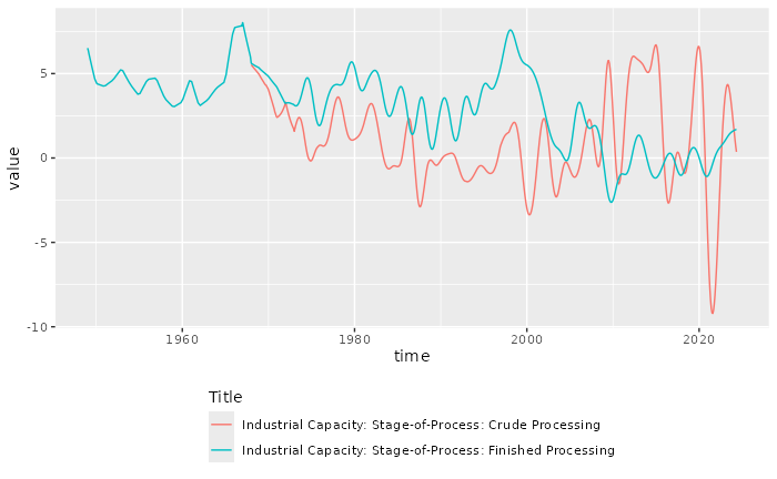
Time series transformations
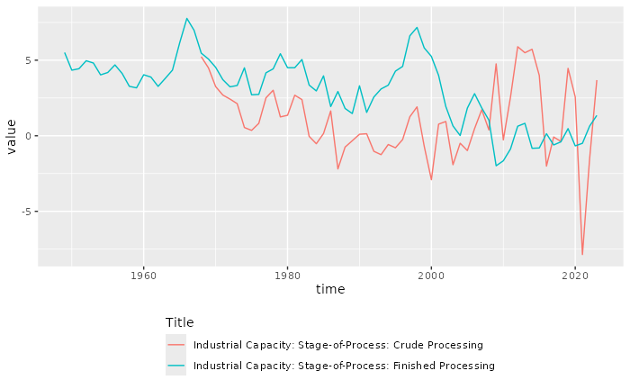
The FRED api also allows some basic time series transformations with
the units parameter:
data_get(c("fred/CAPB5610CS", "fred/CAPB5640CS"), units = "pc1") |>
  drop_na() |>
  ggplot(aes(time, value, color = Title)) +
  geom_line() +
  theme(legend.position = "bottom", legend.direction = "vertical")
#> ⠙ Requesting get
#> ✔ Requesting get [428ms]
#> 
Allowed values for units:
- lin = Levels (No transformation)
- chg = Change
- ch1 = Change from Year Ago
- pch = Percent Change
- pc1 = Percent Change from Year Ago
- pca = Compounded Annual Rate of Change
- cch = Continuously Compounded Rate of Change
- cca = Continuously Compounded Annual Rate of Change
- log = Natural Log
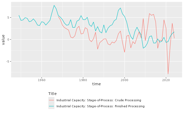
Similarly time series can be temporally aggregated with the
frequency and aggregation_method
parameters:
data_get(c("fred/CAPB5610CS", "fred/CAPB5640CS"), units = "pc1", frequency = "a", aggregation_method = "sum") |>
  drop_na() |>
  ggplot(aes(time, value, color = Title)) +
  geom_line() +
  theme(legend.position = "bottom", legend.direction = "vertical")
#> ⠙ Requesting get
#> ✔ Requesting get [414ms]
#> 
Allowed values for frequency:
- d = Daily
- w = Weekly
- bw = Biweekly
- m = Monthly
- q = Quarterly
- sa = Semiannual
- a = Annual
Allowed values for aggregation_method:
- avg = Average
- sum = Sum
- eop = End of Period